


Today we bring you a guest post. charles angelDonald D. Hester Professor Emeritus of Economics, UW Madison Steve Park Young WooAssistant Professor of Economics at UCSD.
It is generally believed that standard macroeconomic empirical models for exchange rates do not fit the data well (e.g., Miss and Rogoff (1983), Cheung et al. (2005), Itskhoki and Mukhin (2021).) However, we find that these models fit the 21st century US dollar very well.castle century. The “standard” model, which includes real interest rates and expected inflation in the United States and abroad, the U.S. trade balance, global risk, and liquidity demand measures, is well supported by U.S. data on other G10 currencies. The “monetary variables” (i.e., real interest rates and expected inflation) and non-monetary variables play an equally important role in explaining exchange rate movements. Although the fit of the model was poor during the 1970s and early 1990s, model performance has steadily improved to the present. We argue that the improvement was due to better monetary policy (inflation targeting), as the scope for self-fulfilling expectations has disappeared. We provide a range of evidence linking changes in monetary policy to the performance of the exchange rate model.
Here is a link to the working document: here. In this note, we omit technical details and references from the paper. We examine the determinants of the dollar against the euro, British pound, Canadian dollar, Australian dollar, New Zealand dollar, Norwegian krone, and Swedish krona. The Japanese yen and the Swiss franc are special cases that we treat separately.
The empirical model links the monthly changes in the exchange rate between the two countries:
- Real interest rate In the US and “foreign”. Most macro models of exchange rates assume that the higher the real interest rate, the stronger the currency. When US real interest rates rise, the dollar rises, and when foreign real interest rates rise, the dollar falls.
- inflation. Paradoxically, when inflation rises in the US, the dollar rises (and when inflation rises abroad, the dollar falls). This is the conclusion of the New Keynesian macroeconomic paradigm when monetary policy is reliable. When inflation rises (as it has in the past year), the central bank, which targets inflation, tightens. Since we already control for the real interest rate, which is determined by the current stance of monetary policy, this channel captures expectations about future monetary policy actions.
- Trade balance As the trade deficit for U.S. goods and services increases, the U.S. net foreign asset position deteriorates, especially in the early 21st century.castle In the 19th century, markets began to fear that policies would be implemented to weaken the dollar in order to reduce the value of foreign debt, which would lead to a large trade deficit and a depreciation of the dollar.
- Global Risk. The dollar is considered a “safe haven” currency. In times of high global risk (as measured by bond market spreads), the dollar tends to strengthen.
- liquidity. Also, in times of global stress, the market increases its demand for dollar-denominated assets. As demand increases, the “convenience yield” on U.S. Treasury assets increases and the dollar appreciates.
- purchasing power parity. If the relative purchasing power of the dollar is very misaligned, there is a (weak) tendency to revert to PPP levels.
Model estimation
The model is estimated on a currency-by-currency basis and jointly estimated by panel estimation. The macro variables generally have signs and magnitudes consistent with economic theory and are generally statistically significant when estimated from January 1999 to August 2023. (The starting point here was chosen because it corresponds to the advent of the euro.) Figure A, shown here, plots the “fitted values” of the model against the actual exchange rate.
Specifically, the model is estimated for monthly changes in the exchange rate, so the fitted values for the levels shown here are the model’s fitted values for (log) levels of the exchange rate, accumulating the estimated changes in the model each month. The initial value of the accumulator is chosen so that the overall mean of the fitted values is equal to the overall mean of the data.
One thing to be very clear about here is that we are not predicting the exchange rate. The empirical model uses data from, say, January 2000 to explain the exchange rate in January 2000. Even if a macroeconomic model of the exchange rate were a good model, it would not be a useful model for forecasting. Most exchange rates change from month to month due to unexpected changes in the explanatory variables. However, these unexpected changes are by definition unpredictable, so predicting exchange rate changes is very difficult even with the best model.
The model is suitable
Moving on to Figure A, for the EUR/USD exchange rate as an example, the fitted values reproduce well the initial US dollar rally in 1999-2000 and the US dollar decline in 2001-2008. The fitted series also matches the US dollar surge in 2008, 2010, and 2013. Both the data and the fitted series show a dollar rally since 2013. The model-implied series also fits the pattern very well since 2020, mimicking the V-shape for 2021-2023. The close correspondence between the red and blue lines applies to all other currencies in the other sub-periods between 1999 and 2023.
Figure A: Comparison of data and model-embedded exchange rates
The fit has improved over time.
However, this model did not fit the previous sample. We document this by estimating the model on a rolling sample of 20 years starting in 1973. The fit was poor in the previous sample. The variables were generally not statistically significant. Sometimes, when they were significant, they had the wrong sign. R-The square value is low. F– The joint significance test of the explanatory variables failed to reject the null hypothesis. However, it increases almost monotonically. F– Statistics and R2As the sample progresses over time, these statistics essentially peak in the final 20-year sample. Figure B R-square and F Statistics over time in this rolling regression. This shows that the model did not fit well in the initial samples, but the fit steadily improved.
Why this model didn’t work in the past
Why did the initial model fit poorly and now fit so well? We argue that changes in the monetary regime can explain this. As we show, economic theory suggests that when the central bank does not follow a credible inflation targeting policy, there is room for self-fulfilling expectations that affect economic variables, including inflation, output, and the exchange rate. Intuitively, suppose that the market creates a belief that inflation will be higher. If the central bank does not respond strongly enough to this change in expectation, real interest rates will fall. This will stimulate aggregate demand and lead to inflation and a weaker currency. We argue that as credibility increases, this phenomenon decreases and the fit of the standard model improves. When monetary policy is credible, expectations of inflation that suddenly appear out of thin air will not persist, because the possibility of future inflation will quickly disappear as monetary policy tightens.
The fact that the fit improvement is related to the currency variable is clearly shown in Figure C. tea– Statistics on real interest rate variables (Δi, Δi*) and inflation measures (π and π*) obtained from 20-year regression analysis. tea-The statistic measures the contribution of the variables (the estimated regression coefficients) adjusted by the accuracy of the estimates (the reciprocal of the standard error of the estimates), so it gives a good idea of how important each variable is in explaining exchange rate movements. If the theory is correct, this graph shows tea– The statistics should be negative for the U.S. interest rate and inflation variables and positive for the foreign variables. A value of about 2.0 or greater is statistically significant. In Figure C, we see that, with a few exceptions, the variables were rarely significant and often had the wrong sign in the early part of the sample, but became significant with the correct sign in later samples.
The interest rate and inflation variables are important because they indicate whether the exchange rate responds to credible monetary policy. If the policy is credible, a higher real interest rate signals a stronger currency, while a higher inflation rate signals a tighter policy and a stronger currency. This pattern does not hold in the early samples, but it does hold in the later samples.
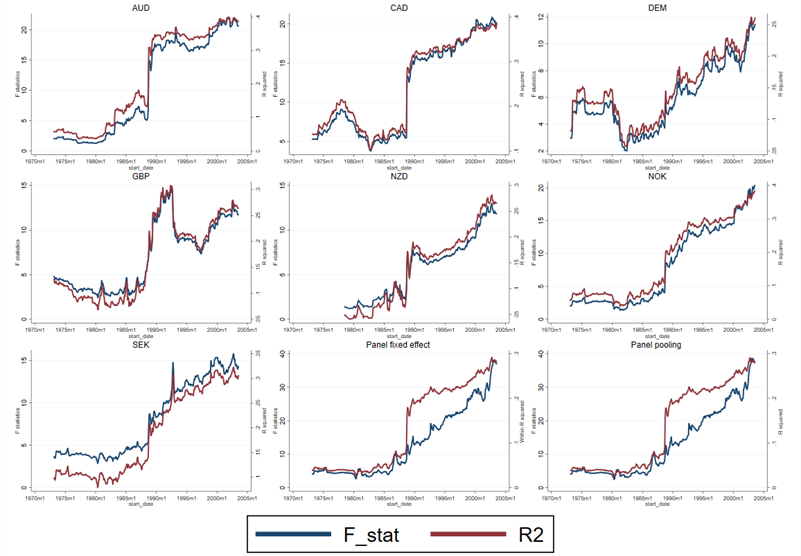
Figure B: F-statistic and R-square for 20-year moving window regression
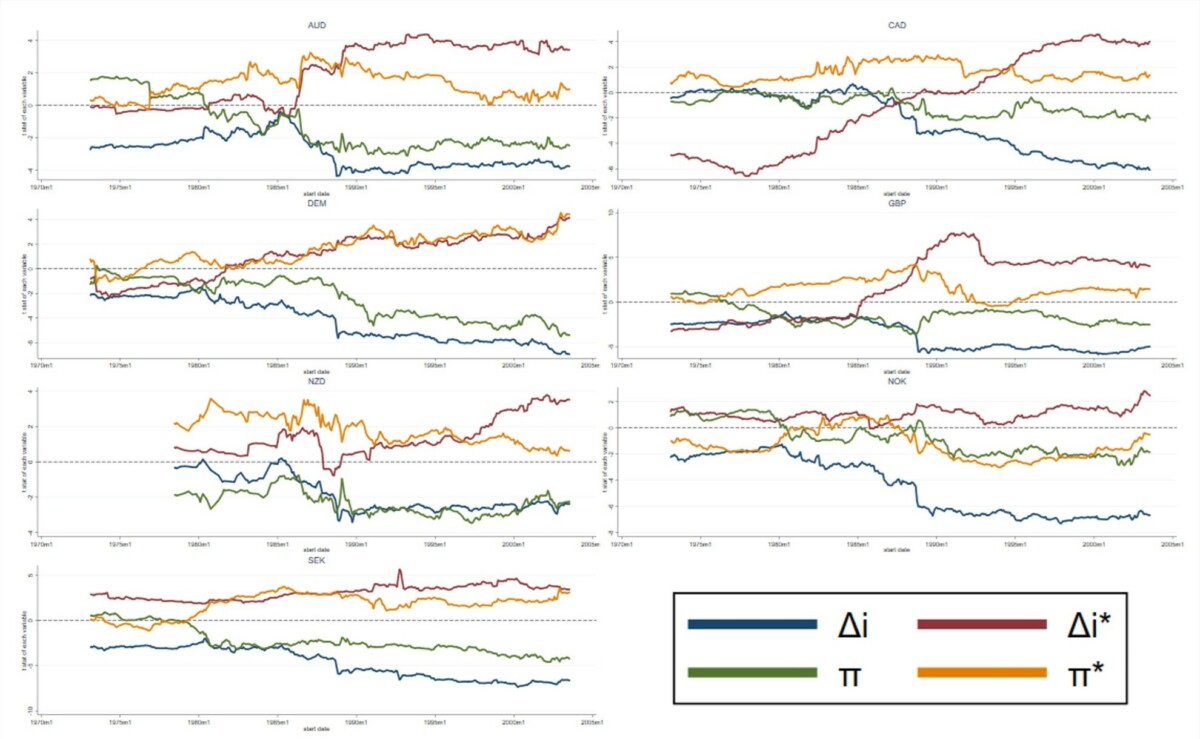
Figure C: t-statistics for 20-year rolling window regression
Since US monetary policy began to change in the Volcker era, the Taylor rule for data starting in the mid-1980s provides support for monetary stability. The advanced economies in the sample adopted inflation targeting a few years later: New Zealand in 1990, Canada in 1991, the UK in 1992, Sweden and Australia in 1993, and Norway in 2001. One of the pillars of the European Central Bank policy since 1999 has been inflation targeting. Germany officially adopted inflation targeting in 1992, before the introduction of the euro, but inflation targeting has always been a core part of Bundesbank policy.
This paper provides additional evidence supporting the shift in monetary policy in these countries and their increasing reliability. The important contribution here is that the success of the empirical model does not depend solely on risk and liquidity variables that are important in tracking dollar movements during times of global financial stress. Variables that represent monetary policy positions in the United States and other countries are important in explaining the fit of the model today and the lack of fit in the past. It is reasonable to attribute these changes over time to the changing nature of monetary policy.
Empirical exchange rate models are better than you think
Clearly, the fit of the model is not perfect. There may indeed be other factors driving the exchange rate, including nonmarket “noise trading” highlighted in recent research. However, the main reason for the imperfect fit is likely that the variables that economists say theory should drive the exchange rate, such as the stance of monetary policy, the level of global risk, and the demand for liquidity, are not perfectly measured. Figure A clearly demonstrates that the empirical model captures the major factors driving the dollar exchange rate.
This post was written by: charles angel and Steve Park Young Woo.


